Introduction to R and RStudio
R Foundations 2024
October 21, 2024
Overview
Why use R?
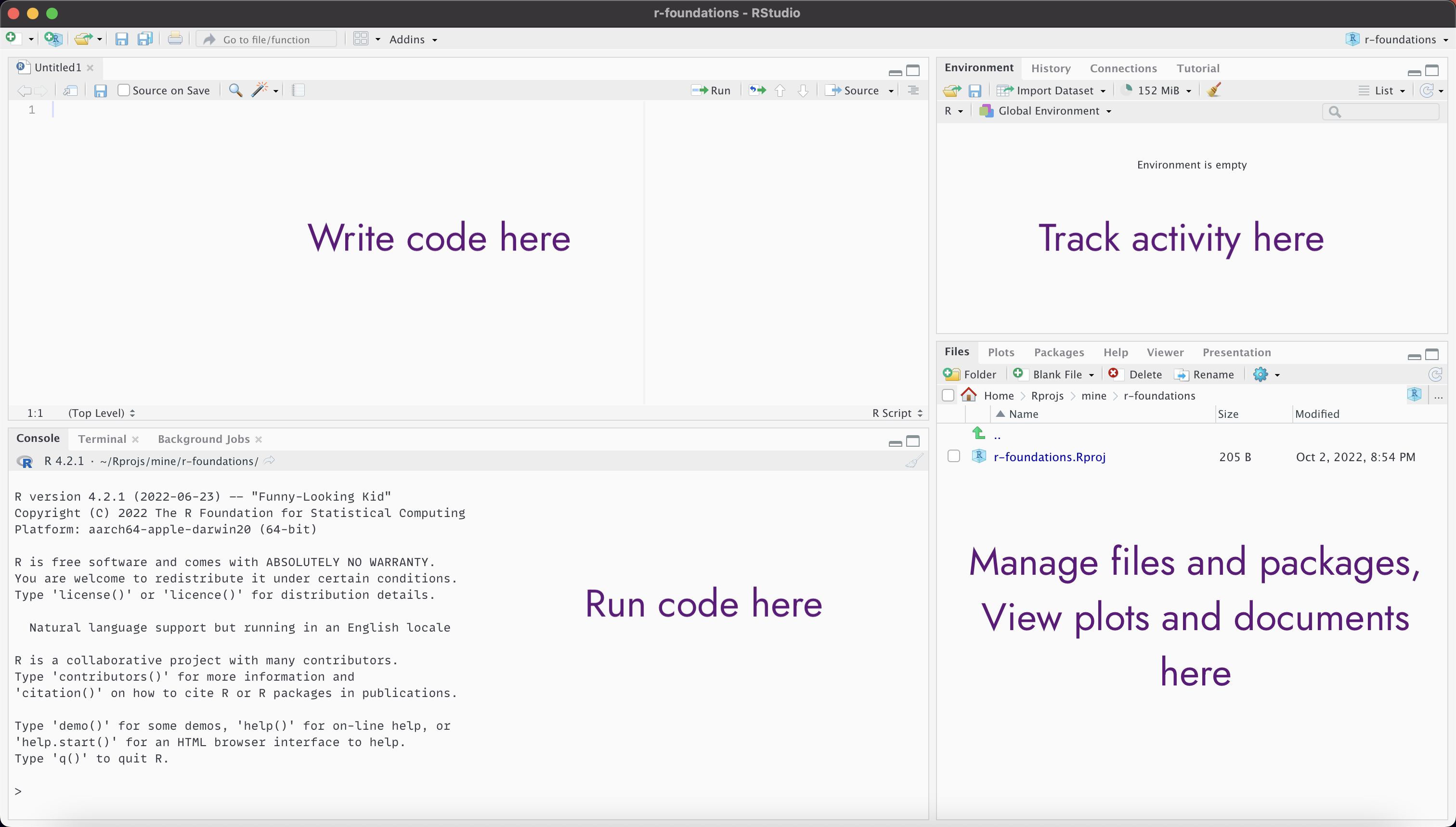
Use RStudio to write and run R programmes
Create and start an R project
Use
install.packages()to install packagesHow to get help in R
See examples of data wrangling and visualisation
Why use R?
What can R do?
Data import
Data management and wrangling
Exploratory data analysis
Statistical modelling
Advanced statistics
Machine learning
Data visualisation
Reports, articles
Dashboards, web apps
Integrates well with other languages
Packages: share your code and use others
The R Ecosystem
Base R
15 base packages
- Create R objects
- Summaries
- Maths functions
- Statistics
- Graphics
- Datasets
15 recommended packages
- Statistics methodology
- More maths
- More graphics
The R Ecosystem
Contributed packages
CRAN
- Official R repository
- https://cran.r-project.org
- nearly 20000 packages
Bioconductor
- Bioinformatics packages
- https://www.bioconductor.org
- ~2100 packages
GitHub
- Packages in development
- GitHub-only packages
The tidyverse
The tidyverse is an opinionated collection of R packages designed for data science. All packages share an underlying design philosophy, grammar and data structures.
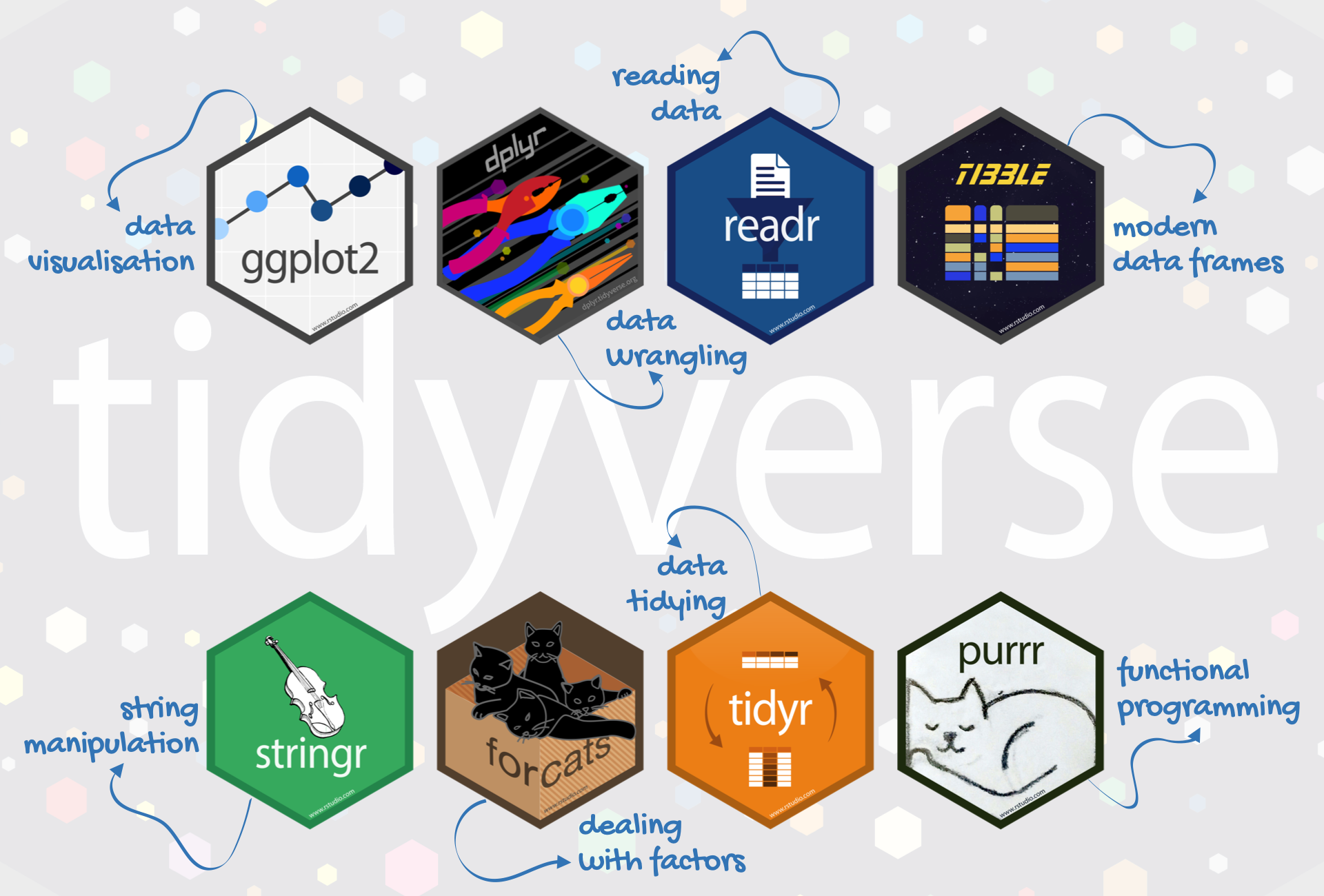
From https://education.rstudio.com/blog/2020/07/teaching-the-tidyverse-in-2020-part-1-getting-started/
tidyverse 2.0.0. includes lubridate for date-times as well (not shown in image).
palmerpenguins
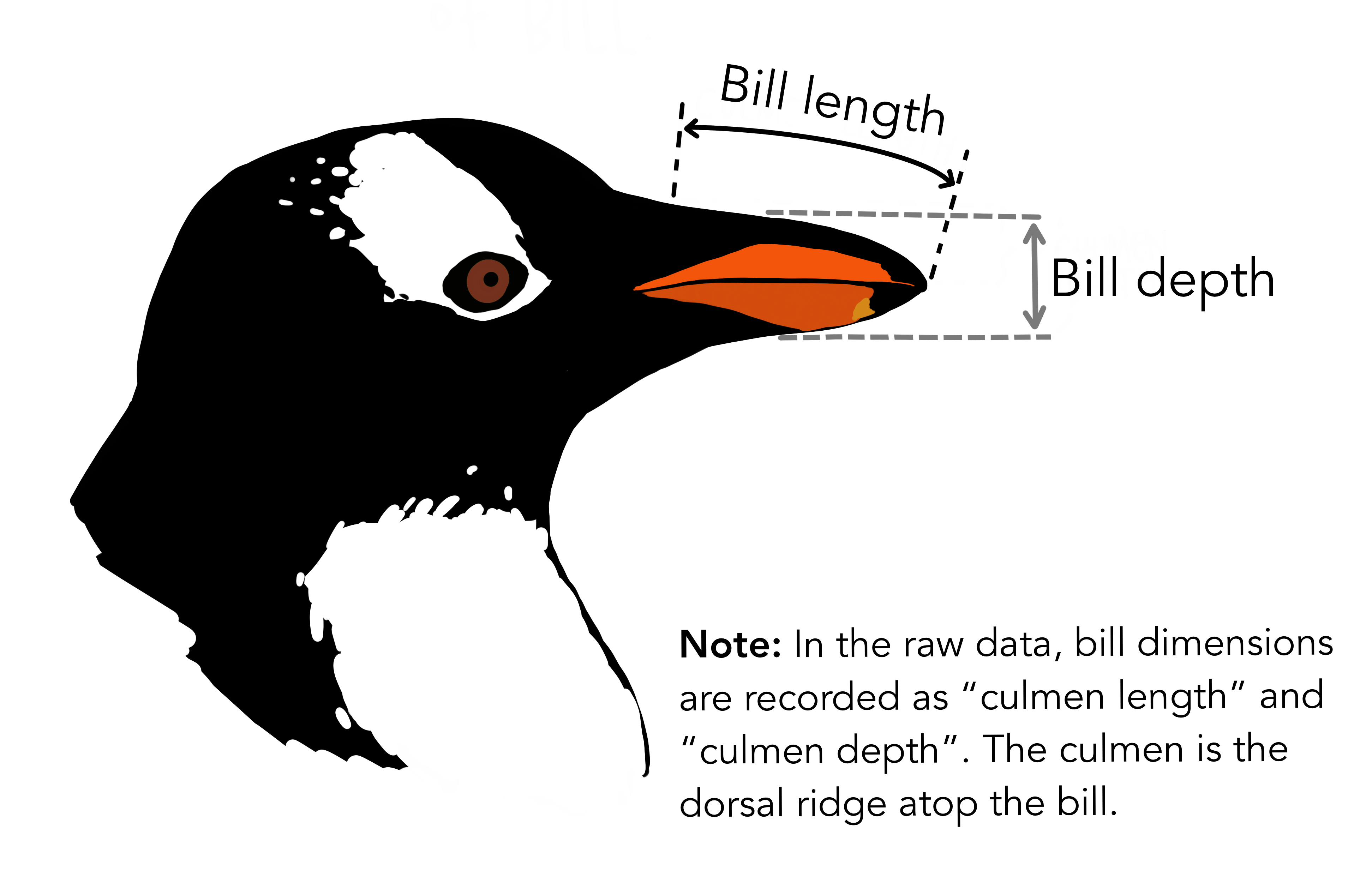
palmerpenguins is a dataset package, designed to be a great example for data exploration and visualisation.
It contains measurement data for 344 penguins, from three different species, collected from three islands in the Palmer Archipelago, Antarctica.

Penguin artwork by Allison Horst https://allisonhorst.github.io/palmerpenguins/articles/art.html
The R community
Another reason to love R is the community around it.
It prides itself on being friendly, diverse, helpful, and supportive.
R user groups, especially Warwick RUG
RLadies, especially RLadies Coventry
#RStats and #TidyTuesday on Mastodon
rainbowR (LGBTQ+)
MiR (minorities in R)
Introducing RStudio
At first
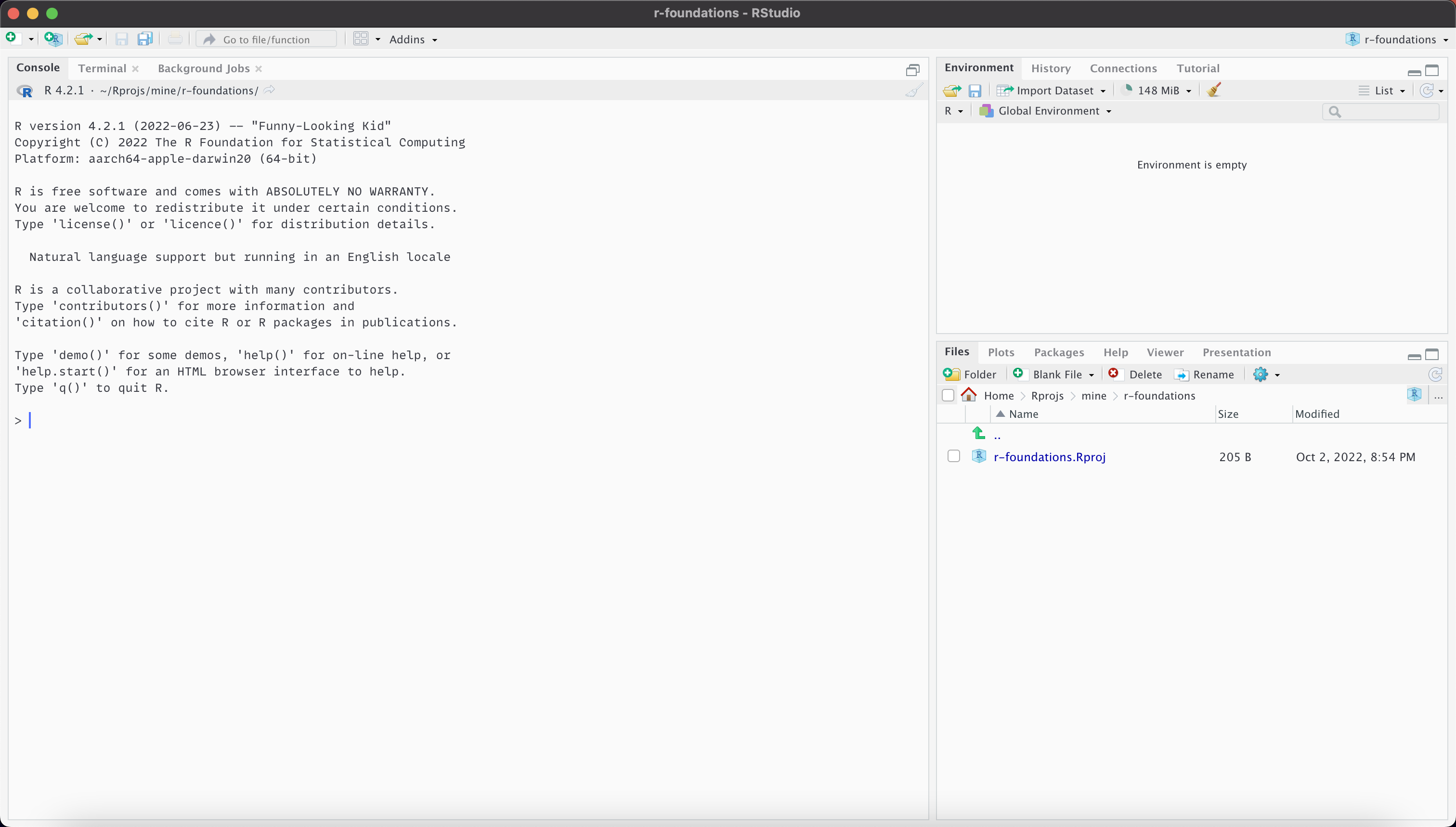
With script
Best practice: use R projects
An RStudio project is a contect for working on a specific project
Keeps files well-organised
Automatically sets working directory to project root
Has separate workspace and command history
Works well with version control via git or svn
Getting started with projects
Create a project from a new or existing directory via the file menu or new project button
Switch project, or open a different project in a new RStudio instance via the project menu
RStudio project demo
Create R-Foundations project
Create first script
Using the console
For things that only need doing once, e.g. installing packages
For doing things you don’t need to track, e.g. requesting help files
To quickly explore new ideas before adding them to a script
Using the console: shortcuts
RStudio provides a few shortcuts to help write code in the R console
- ↑/↓ go back/forward through history one command at a time
- Ctrl/⌘ + ↑ review recent history and select command
- Tab view possible completions for part-written expression
Code completion (using Tab) is also provided in the source editor
Using the console: demo
Using scripts
Text files saved with an .R suffix are recognised as R code
Code can be sent directly from a script to the console as follows:
- Ctrl/⌘ + ↵ or
 run current line
- Run multiple lines by selecting first
- Ctrl/⌘ + Shift + ↵ or

- Run the script from start to finish.
Why R scripts?
Writing an R script for an analysis has several advantages over a graphical user interface (GUI)
- It provides a record of the exact approach used in an analysis
- It enables the analysis to be easily reproduced and modified
- It allows greater control
Good practice for R Scripts
Organising your R script well will help you and others understand and use it.
- Add comment or two at start to describe purpose of script
- Use one or more
#to start a comment
- Use one or more
- Load required data and packages at the start
- Avoid hard-coding: define variables such as file paths early on
- Give functions and variable meaningful names
- use
###or#---to separate sections (in RStudio Code > Insert Section)
Installing packages
In console
Install a package with
install.packages("package_name")- Watch out for the plural!
Install multiple packages with
install.packages(c("package1", "package2"))- The
c()function creates a vector
- The
Or use install button in packages pane:

Loading packages
In script
- Load packages with
library(package_name)
R script demo
Getting help in R
Within R: Help with functions
Within R: help.search
# when ?function_name fails (e.g. don't have package loaded)
help.search("function_name") # note quotation marks
??function_name

# for when you can't quite remember the function name
??something_like_function_name

# R help start page
help.start()
## note that using the RStudio Help home button gives even more resources
Within R: Help with package
# `help`
help(package = "package_name")
# Help panel in RStudio will give links to all documentation
# and help pages for that package

# find/browse vignettes for installed (or specific) packages
browseVignettes()
browseVignettes("package_name")

# use auto-completion in RStudio to see what functions
# are in a package
?package::
dplyr demo
RStudio Help home demo
Your turn
Create an R project called “R-foundations”
Install the packages palmerpenguins and tidyverse
Find the help page for the
penguinsdatasetFind the help page for the
filterfunction in thedplyrpackageExperiment typing commands into the console or in an R script.
link to slides
Getting help at Warwick
What can we learn about penguins?
The data
# A tibble: 344 × 8
   species island    bill_length_mm bill_depth_mm flipper_length_mm body_mass_g
   <fct>   <fct>              <dbl>         <dbl>             <int>       <int>
 1 Adelie  Torgersen           39.1          18.7               181        3750
 2 Adelie  Torgersen           39.5          17.4               186        3800
 3 Adelie  Torgersen           40.3          18                 195        3250
 4 Adelie  Torgersen           NA            NA                  NA          NA
 5 Adelie  Torgersen           36.7          19.3               193        3450
 6 Adelie  Torgersen           39.3          20.6               190        3650
 7 Adelie  Torgersen           38.9          17.8               181        3625
 8 Adelie  Torgersen           39.2          19.6               195        4675
 9 Adelie  Torgersen           34.1          18.1               193        3475
10 Adelie  Torgersen           42            20.2               190        4250
# ℹ 334 more rows
# ℹ 2 more variables: sex <fct>, year <int>
How many of each species?
How many of each species on each island?
Show me the bill dimensions of the 5 heaviest female Gentoo penguins
The native pipe
|> is a pipe.
It passes what comes before into the first argument of what comes after.
Pipes are a powerful tool for clearly expressing a sequence of multiple operations.
We’ll talk more about pipes in the data wrangling session.
What’s the mean bill length, by species?
What’s the relationship between bill length and depth?
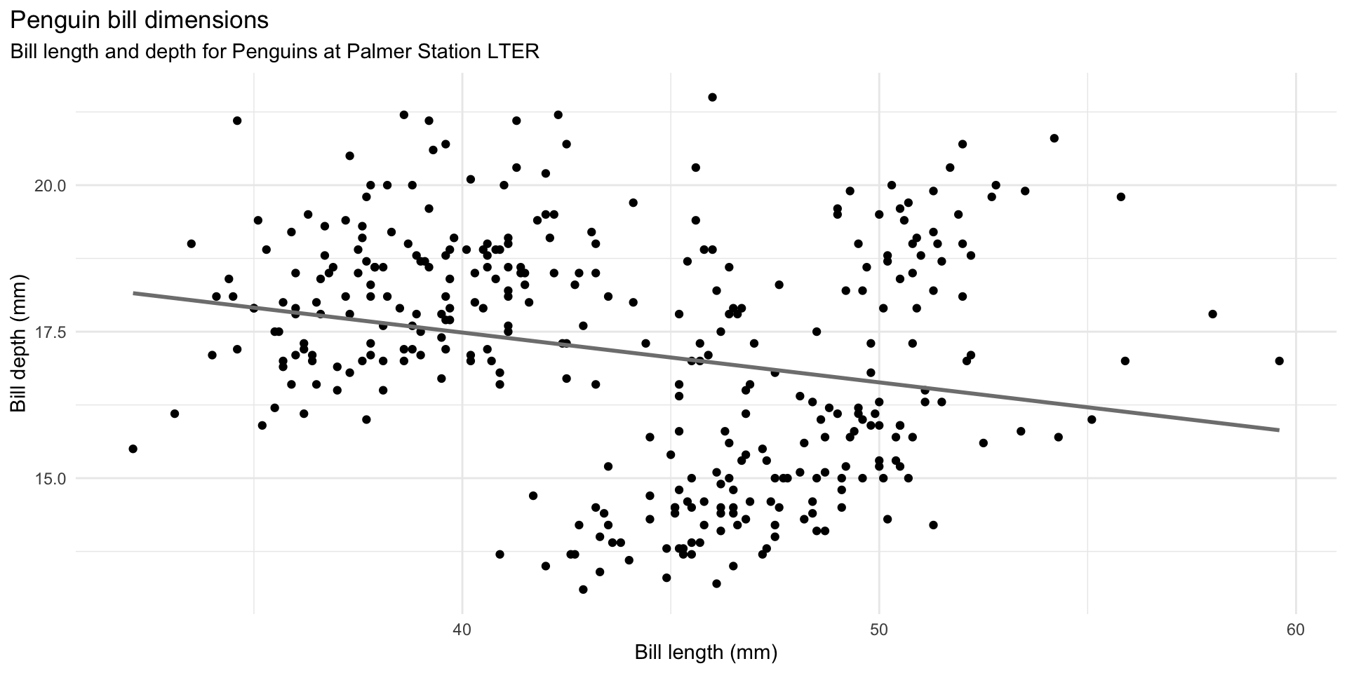
ggplot(data = penguins,
       aes(x = bill_length_mm,
           y = bill_depth_mm)) +
  geom_point() +
  geom_smooth(method = "lm", se = FALSE, color = "gray50") +
  labs(title = "Penguin bill dimensions",
       subtitle = "Bill length and depth for Penguins at Palmer Station LTER",
       x = "Bill length (mm)",
       y = "Bill depth (mm)") +
  theme_minimal() +
  theme(plot.title.position = "plot")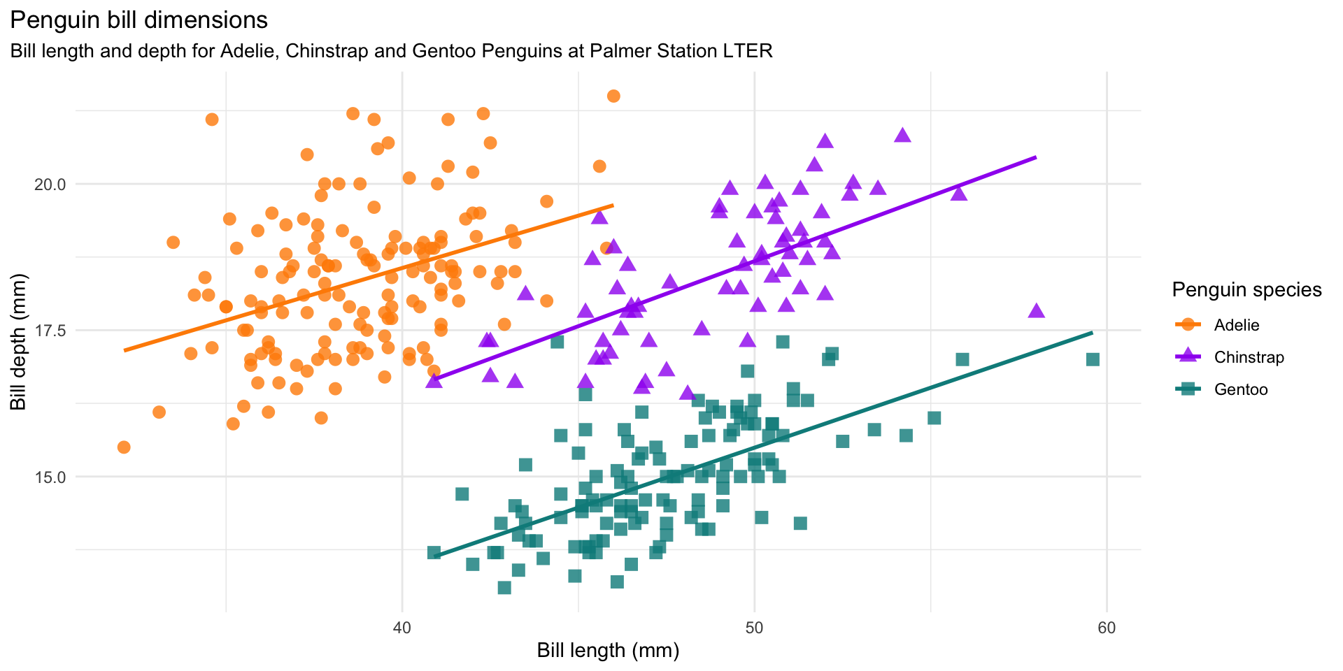
ggplot(data = penguins,
       aes(x = bill_length_mm,
           y = bill_depth_mm,
           group = species)) +
  geom_point(aes(color = species,
                 shape = species),
             size = 3,
             alpha = 0.8) +
  geom_smooth(method = "lm", se = FALSE, aes(color = species)) +
  scale_color_manual(values = c("darkorange","purple","cyan4")) +
  labs(title = "Penguin bill dimensions",
       subtitle = "Bill length and depth for Adelie, Chinstrap and Gentoo Penguins at Palmer Station LTER",
       x = "Bill length (mm)",
       y = "Bill depth (mm)",
       color = "Penguin species",
       shape = "Penguin species") +
  theme_minimal() +
  theme(plot.title.position = "plot",
        plot.subtitle = element_text(size = rel(0.95)))
This is an illustration of Simpson’s Paradox.
Simpson’s paradox is a phenomenon in probability and statistics in which a trend appears in several groups of data but disappears or reverses when the groups are combined.
Example adapted from https://allisonhorst.github.io/palmerpenguins/articles/examples.html
End matter
Resources
Material inspired by and remixed from:
License
Licensed under a Creative Commons Attribution-NonCommercial-ShareAlike 4.0 International License (CC BY-NC-SA 4.0).
